The graphical user interface (GUI)
The graphical user interface lets the user manually examine a drift scan. This is done through a graphical interface that enables a user to select specific locations on the drift scan they would like to fit. The gui also allows the user to view changes made to a drift scan and adjust them accordingly. A walk through of the GUI is given below.
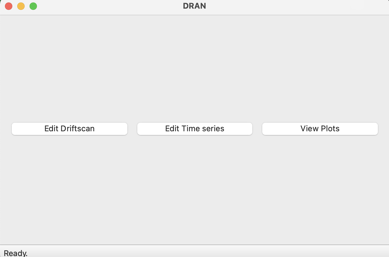
The landing page
The first page you see when the GUI is initiated is the landing page. This page contains the different options the GUI offers with regards to viewing and processing your data. You can edit your drift scan (e.g. perform fitting), edit your timeseries (e.g. manually remove outliers) and view plots of the processed data. A brief summary of each of these options is given below.
Edit driftscan
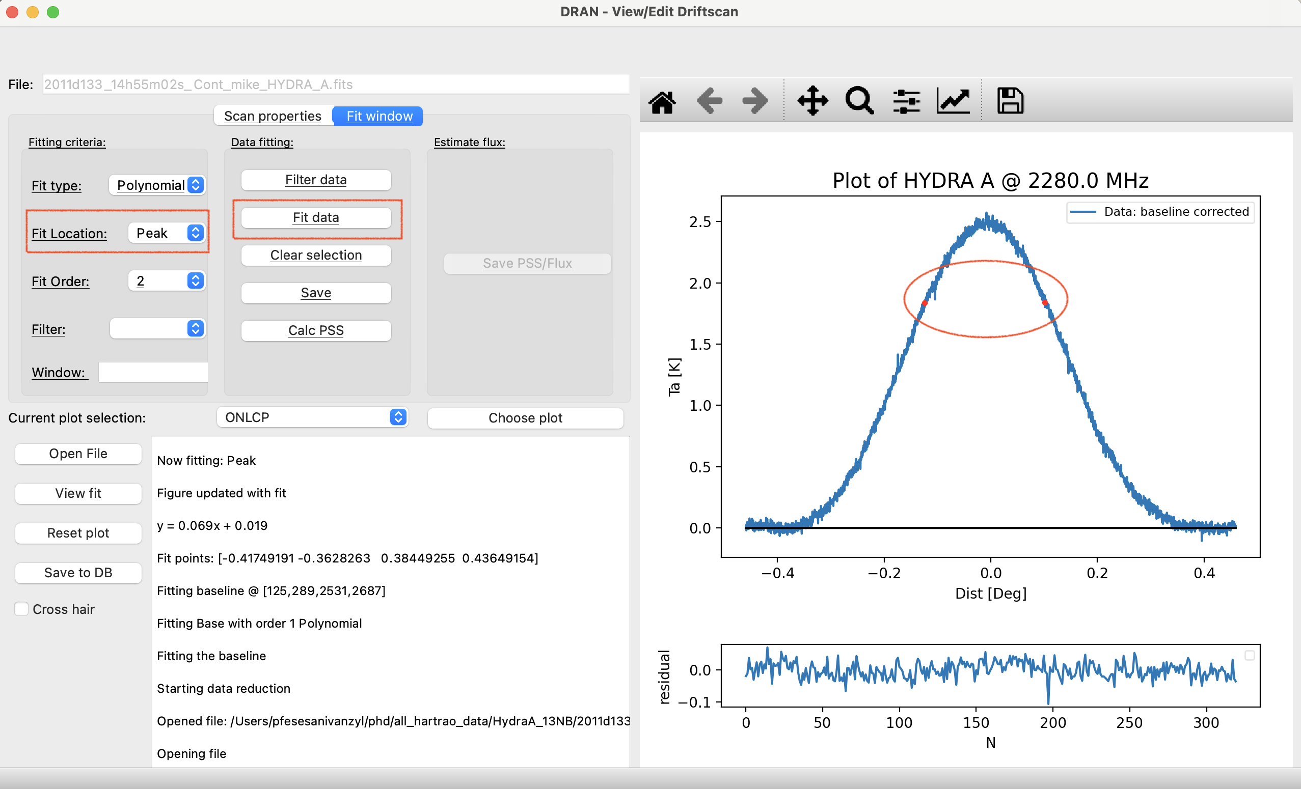
The “Edit Driftscan” button opens up the drift scan editting window. This page shows the basic layout of the GUI. On the left is the “Scan properties” tab, this tab consists of a curated list of some of the drift scan properties found in the drift scan fits file on the observed source. On the second tab, “Fit window”, is information used for the actual fitting. This is currently hidden here but will be shown in the next image. We also have a section to display all the text outputs resulting from running operations on the program, as well as buttons to open a file, view, reset and save drift scan fitting information. On the right is the plot window where the drift scan data is displayed. The next plot shows what the GUI looks like once a drift scan file is opened.

Upon opening a file, the drift scan data is loaded onto the plot window. The top plot displays the current drift scan, and the bottom one is a place holder for the residuals. This operation also toggles the display to the “Fit window” mentioned previously. On this window is the information we need to fit the beam/beams of the drift scan. To toggle between different drift scans we use the “curren plot selection” toggle.
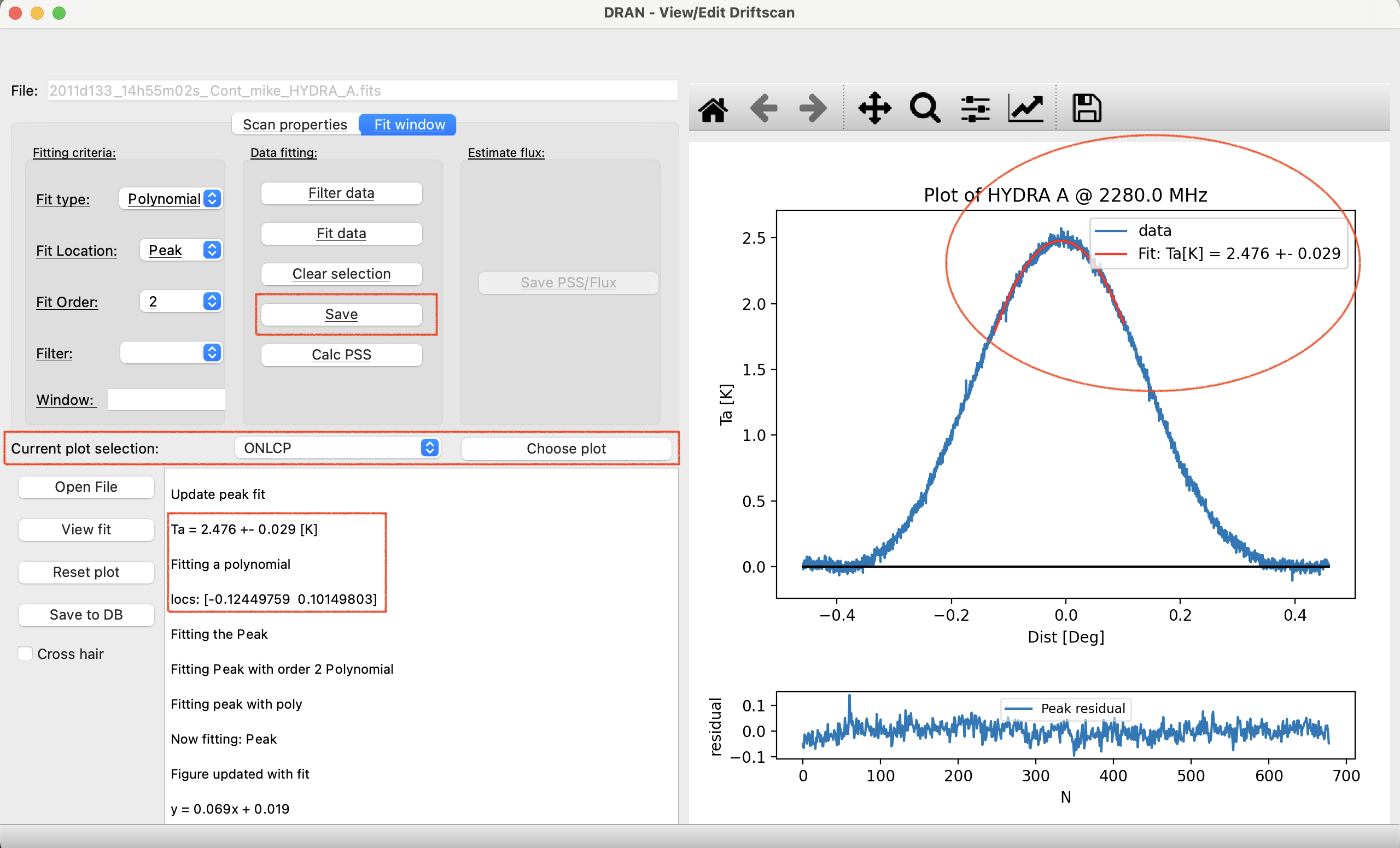
To beginning fitting the drift scan, one can click on the drift scan at the location at which the fit is to be done as shown in the following image.

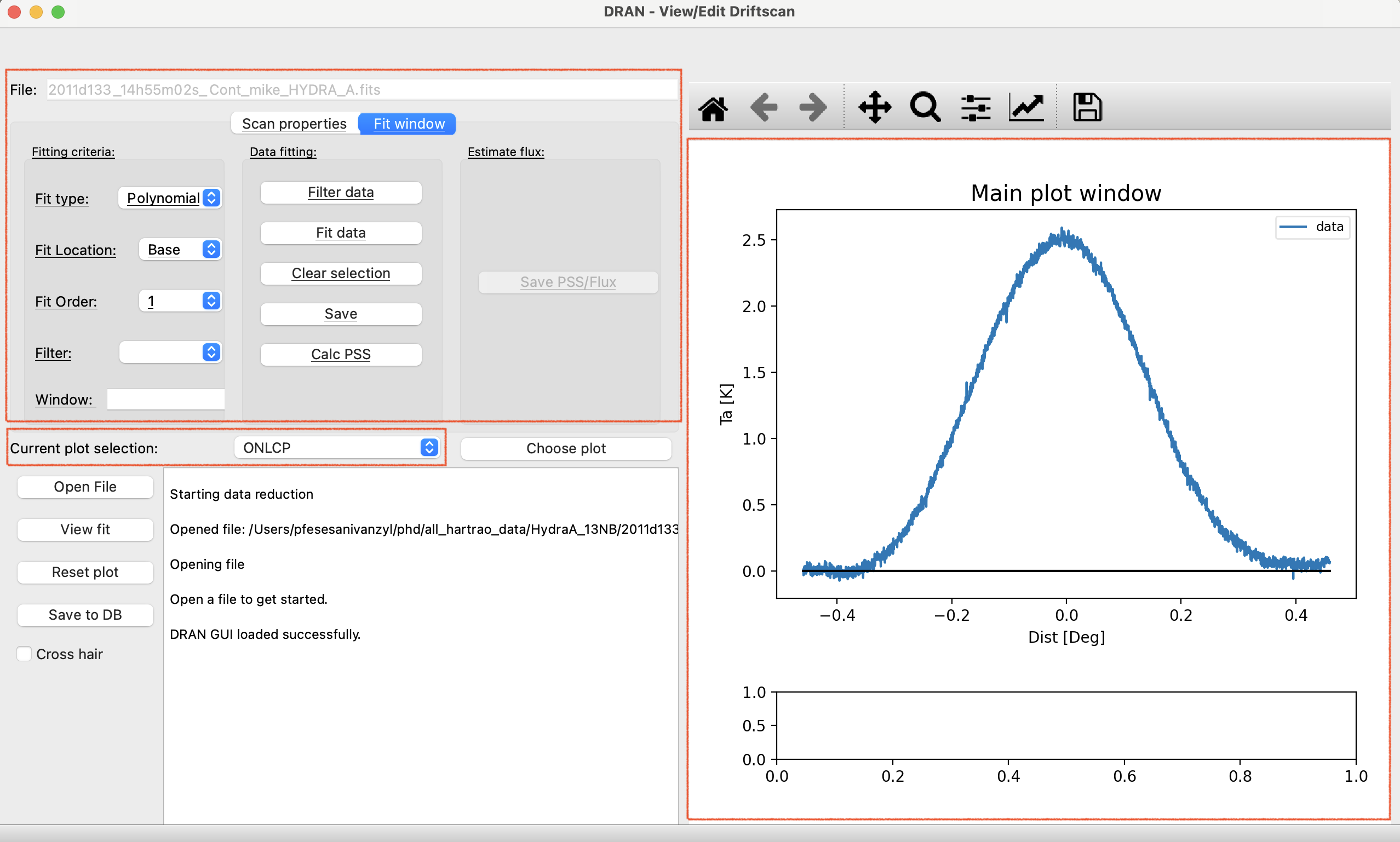
The code is hot wired to process fitting the baseline and peak differently. This is controlled by the “Fit Location” toggle. If you want to fit the baseline, the toggle needs to be on “Base”. Then once you are happy with the locations you clicked on or selected on the plot, you use the “Fit data” button to initiate the actual fit to the baseline blocks selected in the previous step. This creates a new plot with the baseline drift removed as shown below.
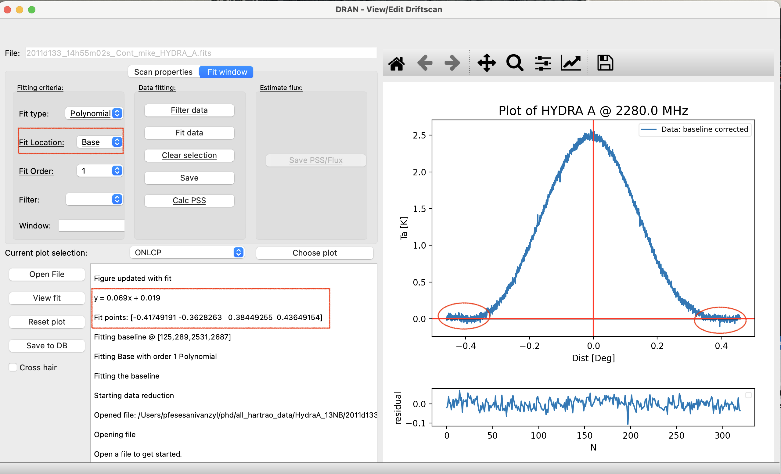
The default baseline fit is a 1st order polynomial, however, this can be adjusted accordingly using the “Fit order” toggle. There are also options to filter the data (smoothing/removing RFI) if needed, with a smoothing window provided to cater for that. After the baseline is corrected the equation of a straight line as well ast the points used for the fit are displayed as well. When fitting the peak, the peak selection works the same way as the baseline selection with the exception that the “Fit Location” toggle is set to “Peak”. Depending on where you want to fit around the peak, you need to select peak fitting points as shown below.
Once you are happy with the selection points, you press “Fit data” again so the program fits the peak of the corrected data. This will create a new fit overlayed on the plot with information on the peak fit and its error. It is this value that we use to calculate the PSS or the source flux depending on the target object under investigation.
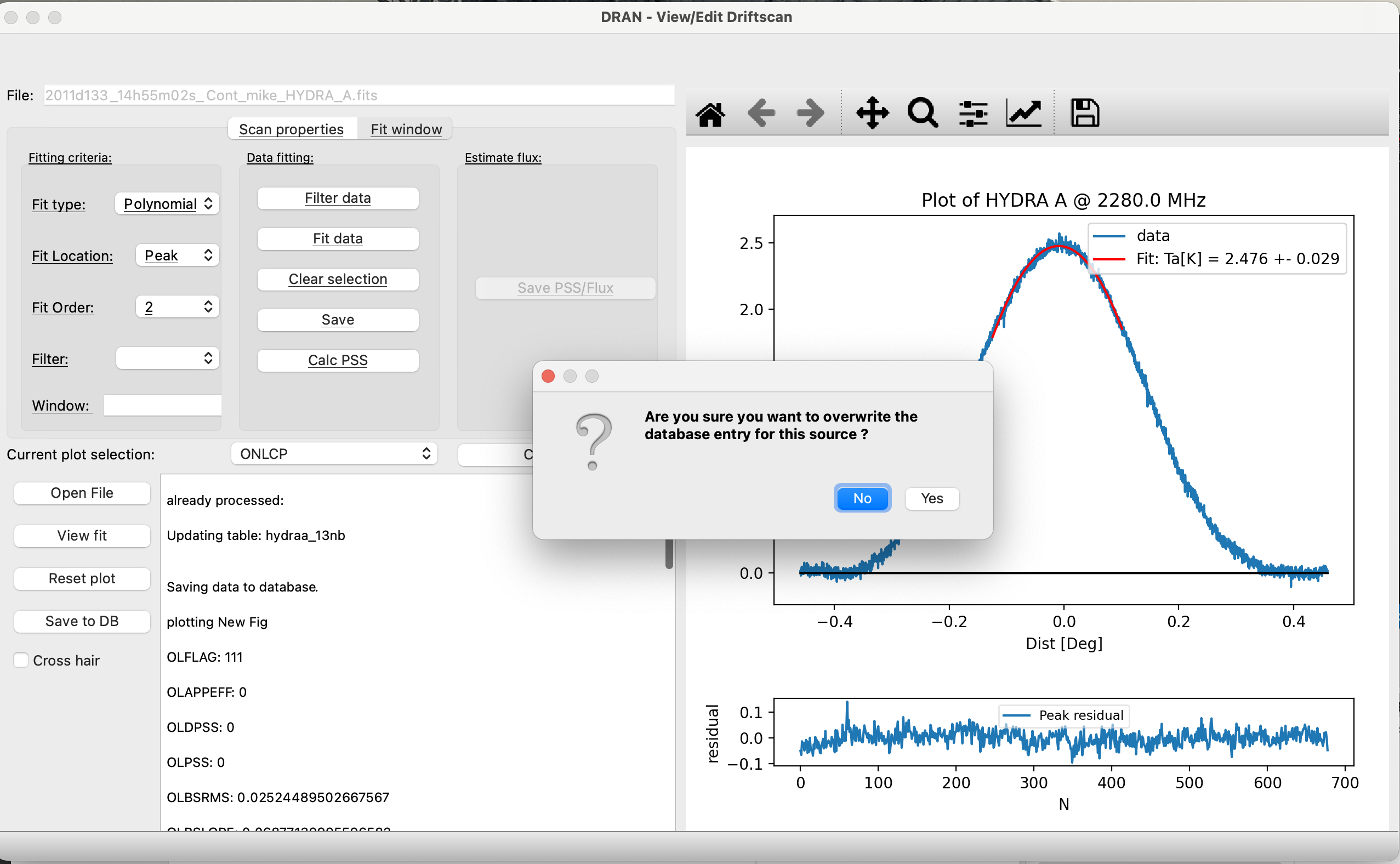
When you are happy with the fit, you need to save it using the “Save” button. This saves the changes made to the current session, in this example, we are saving changes made to the LCP ON SCAN drift scan. The minute you press save, any previous data you had previously processed on this observation for this scan will be replaced by the changes you made. This will also update the previous image you had. If you want to make changes to other sessions as well you can use the “Current plot selection” toggle to change to new drift scan session and load a different set of data. It is imperative to remember that for any changes to be save you need to click on the “Save” button for each session or each different drift scan. To view the values that will be modified on the database, click on “View fit”. At this point the changes are still local to your session, so to make the changes permanent on the database you need to click on “Save to DB”. This updates the database and makes your changes permanent. A popup will appear and ask if you are sure you want to continue modifying the values in the database, If you are, you click yes and end your session. If you want for example to revert to the previously automated fit that you accidentally modified using the GUI, you need to go into the database and delete the observation from there, then run the code again in automated mode to re-process the automated fit.
Edit Time series
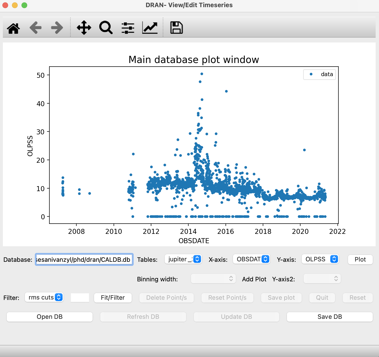
Currently this feature is not fully operational. The plan is to have this gui allow you to modify timeseries data manually. Right now, all you can do is view the timeseries data and view the drift scan plots responsible for the points on the time series data.
Opening a database in “Edit Time series” lets you plot any timeseries on the data provided. For this example I’m plotting observed date vs PSS.
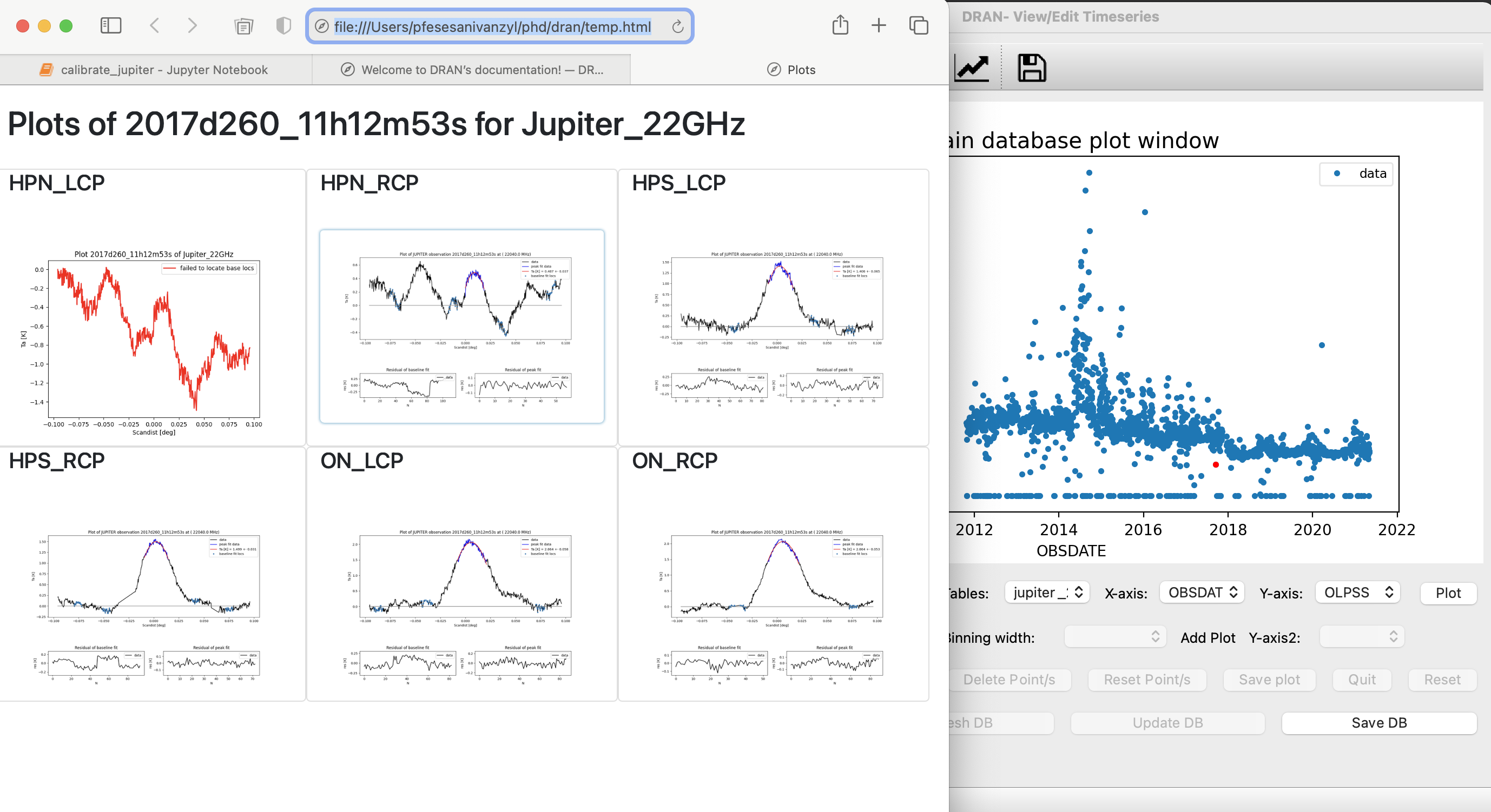
To view the drift scan plots that provided a specific point on the timeseries you click on the point in the timeseries and a popup html will show up with all the processed scans for that specific point.
Note
In future releases the GUI will be adapted to also handle timeseries analysis.
View plots
View plots lets you view the thumbnails of all the plots made by the code for each observed object.
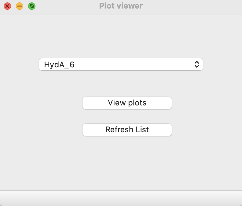
Selecting the object name from a dropdown list provies a tile view of all the plots made for that current object. Clickin on the tiles provides a zoomed in image of the thumbnail.
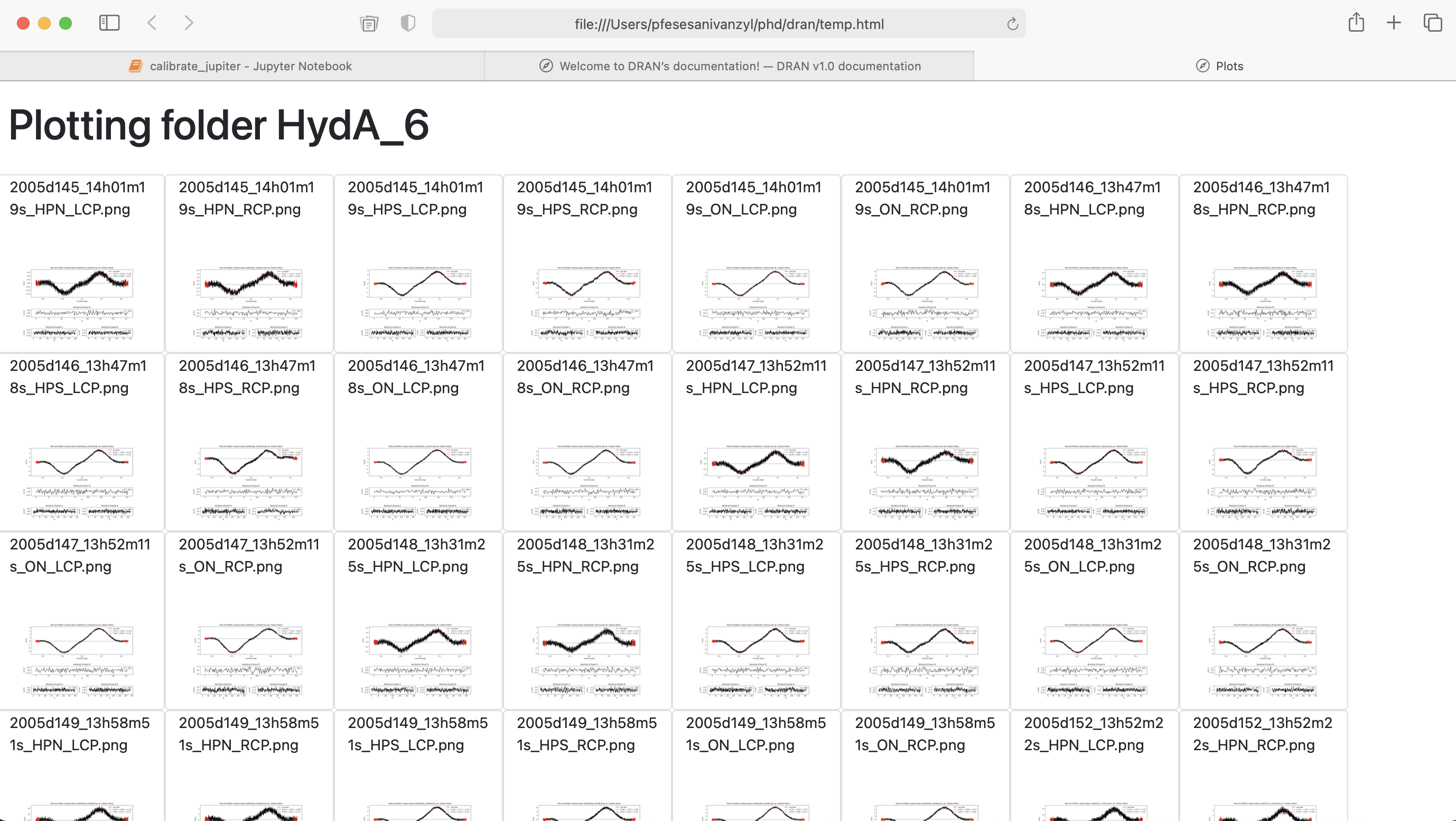
Currently this does not work well when there is a lot of data because the page takes a long time to load. In future work this will be modified for effecient page loading.